
Central idea: radiance is the quantity that carries source brightness through an optical system. Detector power appears only after radiance is integrated over the area, angles, wavelength band, and transmission actually accepted by the measurement.
From source to signal
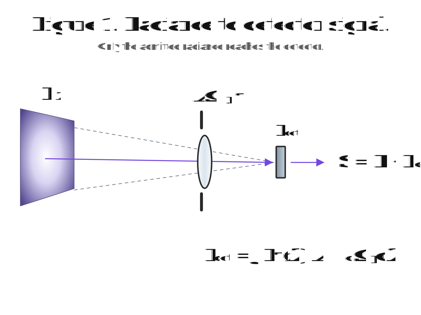
One equation organizes the entire problem
Many detector calculations begin too late. A measured voltage is divided by a responsivity, or a blackbody temperature is inserted into Planck's law, before the optical geometry has been made explicit. The more reliable starting point is the spectral power that actually crosses the detector surface.
For incident spectral radiance \(L_\lambda(\mathbf r,\hat{\mathbf s})\), the spectral power received by a detector is
where \(A_d\) is detector area, \(\Omega_{\mathrm{acc}}\) is the accepted set of incoming directions, \(\theta\) is the angle between an incoming ray and the detector normal, and \(\tau_\lambda\) represents the wavelength- and angle-dependent transmission of the optical path.
The detector then performs a second spectral weighting. For current responsivity \(R_I(\lambda)\),
and similarly for voltage responsivity \(R_V(\lambda)\).
The useful separation is physical: radiometry determines how much spectral power arrives. Responsivity determines what the detector does with that arriving power. Mixing those steps makes geometry errors look like detector-performance errors.
Radiance, irradiance, exitance, and flux are different questions
The terminology becomes much easier if each quantity is tied to the question it answers.
| Quantity | Typical symbol | Question | SI units |
|---|---|---|---|
| Radiant flux / power | \(\Phi\) | How many watts cross the boundary? | W |
| Irradiance | \(E\) | How much incoming power arrives per unit receiver area? | W m\(^{-2}\) |
| Radiant exitance | \(M\) | How much outgoing power leaves a source surface per unit source area, integrated over the outward hemisphere? | W m\(^{-2}\) |
| Radiant intensity | \(I\) | How much source power is emitted per unit solid angle? | W sr\(^{-1}\) |
| Radiance | \(L\) | How much power is carried per unit projected area and per unit solid angle? | W m\(^{-2}\) sr\(^{-1}\) |
| Spectral radiance | \(L_\lambda\) | How is that radiance distributed with wavelength? | W m\(^{-2}\) sr\(^{-1}\) m\(^{-1}\) |
For infrared detector work, radiance is usually the most useful source-side quantity because it retains both spatial and angular information. Exitance has already integrated over the source hemisphere. Irradiance has already integrated over the set of directions reaching the receiver.
The two integrations have the same structure:
Exitance asks how radiance leaves a surface. Irradiance asks how radiance arrives at a surface.
Terminology: this article uses radiant exitance for \(M\) and emissivity for the dimensionless material property \(\epsilon\). The word emittance appears in some thermal-radiation literature, but "exitance" avoids ambiguity.
A blackbody gives radiance, not detector power
For an ideal blackbody, Planck's law gives spectral radiance
with \(\lambda\) expressed in meters if the SI form above is used directly. For an ideal blackbody, \(L_\lambda=B_\lambda\). A real source is usually described by a spectral emissivity, so a first approximation is
with additional reflected-background terms included when the source emissivity is not close to unity or when the surrounding radiance is significant.
For a Lambertian blackbody, radiance is independent of emission direction. Integrating over the outward hemisphere gives
After integrating over wavelength,
The factor is \(\pi\), not \(2\pi\), even though a hemisphere contains \(2\pi\) steradians. The missing factor comes from projection: rays emitted close to the surface plane contribute less flux through the surface because of the \(\cos\theta\) weighting.
This is more than a blackbody identity. The same cosine-weighted angular integral that gives \(M=\pi L\) also determines the irradiance received by a detector from any finite acceptance cone. The unifying quantity is projected solid angle.
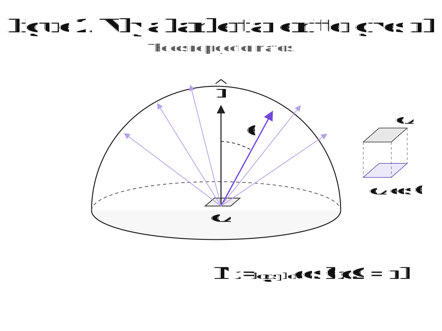
Solid angle is necessary; projected solid angle is what enters flux
A geometric solid angle \(d\Omega\) describes angular extent. For a small planar element \(dA\) seen from distance \(r\),
For a circular cone with half-angle \(\alpha\), the geometric solid angle is
But detector irradiance contains another cosine projection at the receiving surface. It is therefore useful to define the projected solid angle
For an axisymmetric cone,
If a uniform radiance \(L\) completely fills that cone, the received irradiance is simply
In the small-angle limit,
This is why the common shorthand \(E\approx L\Omega\) works well for narrow cones but becomes increasingly inaccurate for wide angular acceptance.
For an on-axis circular disk of radius \(a\), viewed from distance \(r\), the disk edge defines \(\alpha=\tan^{-1}(a/r)\), so
When \(a\ll r\), this becomes
The familiar inverse-square dependence has now appeared, but notice where it came from: the source radiance did not decrease with distance; the source occupied a smaller angular region of the detector's view.
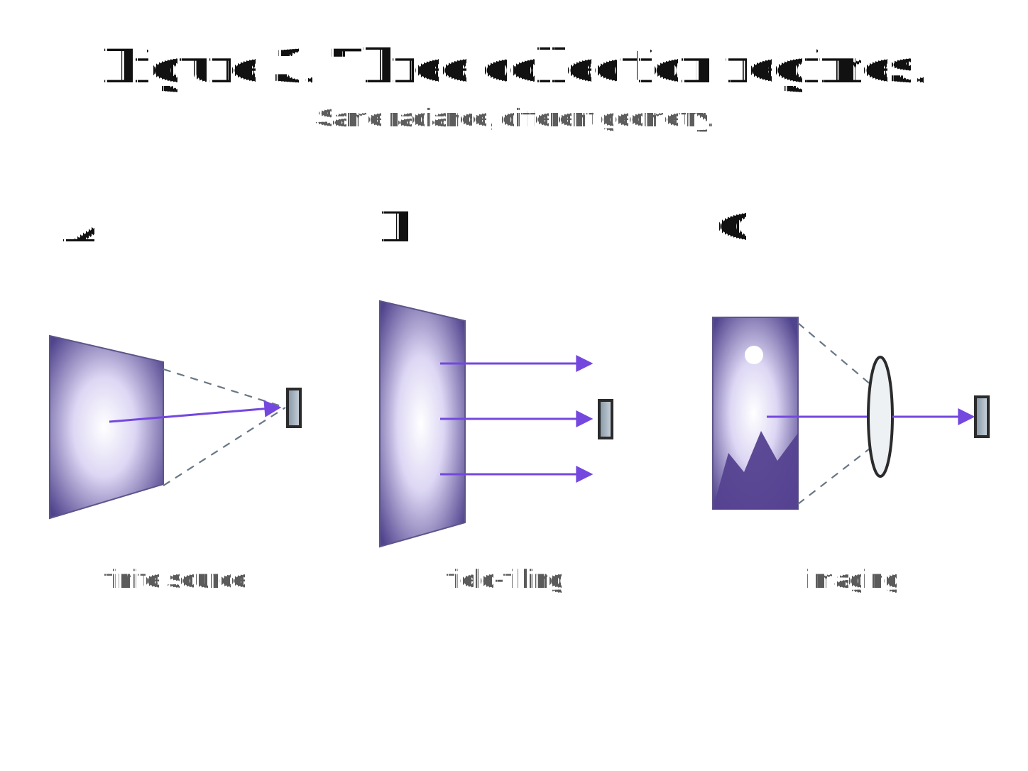
Three collection regimes explain most detector-bench confusion
Statements such as "signal follows \(1/r^2\)" or "image brightness is independent of range" can both be correct. They refer to different radiometric regimes.
1. Finite source viewed by a bare detector
For a small, parallel, on-axis source and detector separated by \(r\), with both dimensions small compared with the separation,
The detector intercepts less power at greater distance because the source subtends a smaller solid angle. This is the regime in which inverse-square reasoning is appropriate.
2. Uniform extended source filling the detector's accepted angular field
If the accepted angular cone is completely filled by a uniform source,
Distance does not explicitly appear. If the source remains large enough to fill the accepted field as it moves, the detector can receive essentially the same irradiance even though the physical source is farther away.
3. Extended source imaged onto a detector or focal plane
An imaging system maps scene radiance to image-plane irradiance. For a scene patch that fills the relevant detector IFOV, image irradiance is controlled primarily by scene radiance, optical transmission, and the aperture cone represented by numerical aperture or f-number—not by a simple source-to-detector inverse-square law.
Once the target becomes smaller than the detector IFOV or pixel footprint, its finite angular size matters again, and signal begins to fall with shrinking target solid angle.
The regime transition is the important part. Range independence applies only while an extended source continues to fill the spatial/angular mode being measured. When it stops filling that mode, the \(1/r^2\)-like angular dilution reappears.
Field of view and acceptance cone are not the same thing
This distinction is often blurred in detector discussions.
Field of view (FOV) describes which scene directions are mapped into the detector or focal plane. For a single pixel, the relevant quantity is often the instantaneous field of view (IFOV).
Acceptance cone describes the range of ray directions from a given scene point that the aperture allows to converge onto a detector location. In an imaging system, that cone is characterized by numerical aperture or f-number.
They answer different questions:
| Quantity | Controls | Typical consequence |
|---|---|---|
| FOV / IFOV | Which part of the scene contributes | Target occupancy, spatial background, scene coverage |
| NA / f-number | How large a ray cone is accepted from each resolved scene element | Image irradiance, throughput, diffraction scale |
| Cold stop / aperture stop | Which pupil directions are physically admitted | Background control, stray-light rejection, throughput |
A wide FOV does not automatically mean a fast optical system. A narrow-FOV system can still have a large numerical aperture. Conversely, a wide-angle imager can be optically slow.
For a bare detector behind a simple tube or aperture, the two concepts may collapse into nearly the same geometric cone. In an imaging system they should be kept separate.
Étendue is the phase-space budget
Area alone does not describe optical collection. Solid angle alone does not either. Their product is the more fundamental throughput quantity.
A general form of optical étendue is
and for a uniform planar area in a narrow cone,
In air and for a circular acceptance cone, a more exact on-axis form is
Étendue is useful because it packages the spatial and angular acceptance into a single optical-throughput budget. An ideal passive optical system cannot arbitrarily compress both area and angle. In a uniform refractive index, lossless geometrical optics conserves radiance along the ray bundle; across refractive-index changes, the invariant is \(L/n^2\), consistent with conservation of étendue.
This puts a hard constraint behind familiar engineering tradeoffs. A lens can make a spot smaller, but doing so increases the angular spread. A smaller detector can be used, but the required numerical aperture rises if the same throughput is to be preserved. Passive optics can redistribute the phase-space volume; they cannot create radiance.
Detector interpretation: when two test setups produce different signal on the same detector, the difference may be an \(A\Omega\) difference rather than a detector-responsivity difference. Normalizing by detector area while ignoring angular acceptance is incomplete whenever the optical throughput differs.
f-number is radiometry written in imaging language
The projected-solid-angle result connects directly to a camera or infrared imaging system.
Suppose an extended scene with radiance \(L\) is imaged through optics with transmission \(\tau\). If the detector sees a circular image-space cone with half-angle \(u'\), the on-axis image irradiance is
For a paraxial system in air,
where \(N=f/\#\) is the relevant f-number. Therefore,
for the idealized on-axis, extended-source case.
This is one of the most useful radiometric relations in infrared imaging:
Changing from \(f/4\) to \(f/2\) increases ideal image irradiance by a factor of four, assuming transmission and other conditions remain unchanged.
For finite-conjugate systems, the working f-number should be used rather than blindly inserting the infinity-focus f-number. Real pupils, obscurations, aberrations, and wavelength-dependent transmission also modify the result.
Where the cosine-to-the-fourth law belongs
The classical cosine-fourth law describes off-axis image-irradiance roll-off for an idealized thin imaging lens. In its common form,
where \(\theta\) is the field/chief-ray angle used by the idealized geometry.
| Off-axis angle | \(\cos^4\theta\) | Ideal relative irradiance |
|---|---|---|
| \(0^\circ\) | 1.000 | 100% |
| \(15^\circ\) | 0.871 | 87.1% |
| \(30^\circ\) | 0.563 | 56.3% |
| \(45^\circ\) | 0.250 | 25.0% |
| \(60^\circ\) | 0.0625 | 6.25% |
Conceptually, the roll-off comes from how projected pupil area, ray obliquity, and image mapping change off axis. It is not a universal detector angular-response law.
Do not apply \(\cos^4\theta\) indiscriminately. The classical law is an approximation associated with a thin, slow, aberration-free lens with a simple stop geometry and no vignetting. Real systems may depart substantially because of pupil aberration, telecentricity, mechanical vignetting, distortion, filter-angle effects, detector angular response, or intentionally designed illumination correction.
The useful practical distinction is:
- Detector angular responsivity is a property of the detector package, absorber, cavity, coatings, and incidence geometry.
- Cos-fourth image roll-off is an optical-system effect.
- Mechanical vignetting is a separate loss mechanism that can further reduce off-axis flux.
FOV and throughput also set the background load
Infrared detectors do not receive only target radiance. They receive every radiance component admitted by the optical system: target, atmosphere, warm optics, enclosure walls, windows, filters, shields, and stray paths.
For a uniform background radiance filling the accepted cone, the background power is approximately
when the detector area and angular acceptance can be treated independently.
The corresponding photon arrival rate is
Increasing throughput can therefore improve target signal and simultaneously increase background loading. In a background-limited infrared system, the relevant design question is not simply "How can I collect more light?" It is "How can I collect more useful target radiance relative to the background radiance admitted into the same optical modes?"
This is the radiometric reason cold shields, cold stops, spectral filters, baffles, and controlled FOV are central to infrared detector systems.
FOV is a signal-to-background parameter, not just an imaging parameter. If the target already fills the required spatial field, widening the admitted field may add little target signal while adding substantial warm-background power.
Worked example: a 500 K blackbody and a small infrared detector
Consider a deliberately simple free-space measurement:
- blackbody temperature: \(T=500\ \mathrm K\)
- circular source aperture diameter: \(25\ \mathrm{mm}\)
- source-to-detector distance: \(250\ \mathrm{mm}\)
- detector active area: \(0.25\times0.25\ \mathrm{mm^2}\)
- spectral band: \(8\text{–}12\ \mu\mathrm m\)
- band-independent optical transmission for this example: \(\tau=0.70\)
- parallel, on-axis source and detector surfaces
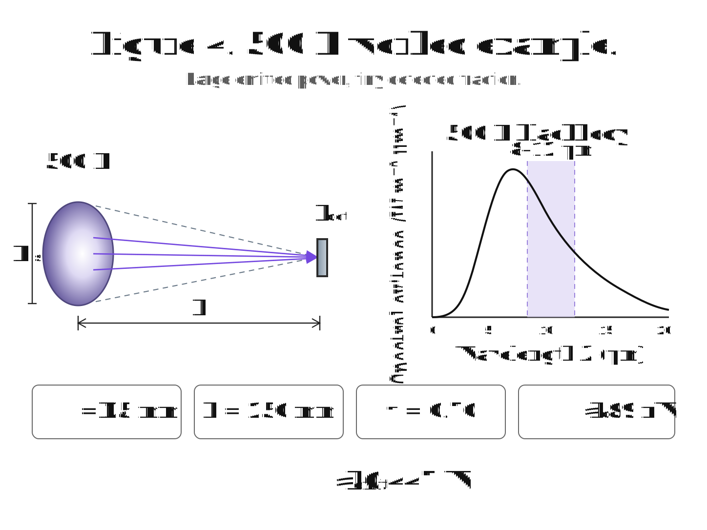
Step 1: total blackbody exitance
The source aperture area is
So the aperture emits approximately
into the outward hemisphere when integrated over all wavelengths.
That 1.74 W is not the detector input power. It is the total hemispherical emission from the aperture.
Step 2: restrict the calculation to the 8–12 µm band
Integrating the 500 K Planck spectral radiance over \(8\text{–}12\ \mu\mathrm m\) gives approximately
The corresponding band-limited hemispherical exitance is
Thus the 25 mm aperture emits about
into the hemisphere in this spectral band.
Step 3: calculate the angular coupling to the detector
The source radius is \(a=12.5\ \mathrm{mm}\), so the cone half-angle at the detector is
The projected solid angle of the circular source at the detector is
Step 4: calculate band-limited detector power
The detector area is
Using the integrated band radiance, projected solid angle, and 70% transmission,
The difference is about \(4.5\times10^6\) in this example. Nothing mysterious happened to the missing power. Nearly all of it simply occupied directions and areas that the detector did not accept.
Step 5: only now convert optical power into electrical signal
If a detector had a flat current responsivity of \(R_I=1\ \mathrm{A/W}\) across this band purely for illustration, the corresponding current would be
A real detector calculation should instead use the measured \(R_I(\lambda)\) or \(R_V(\lambda)\) and perform the spectral integral. The example is intentionally arranged to show the order of operations:
Common radiometric failure modes in detector characterization
- Using \(\sigma T^4\) as detector irradiance.
Stefan–Boltzmann gives blackbody radiant exitance. Geometry and angular acceptance still have to be applied. - Using \(2\pi L\) instead of \(\pi L\) for a Lambertian hemisphere.
A hemisphere contains \(2\pi\) sr, but flux through a surface is cosine weighted. The projected hemispherical solid angle is \(\pi\). - Using geometric solid angle when projected solid angle matters.
For small cones the difference is negligible; for wide cones it is not. - Assuming inverse-square loss in every optical configuration.
It applies naturally to finite angular sources. It does not describe the image irradiance of a resolved extended source that continues to fill a detector IFOV. - Treating FOV and f-number as interchangeable.
FOV selects scene directions. f-number sets the aperture cone and therefore image-plane throughput. - Normalizing by detector area but not by optical throughput.
Two systems with the same detector area can admit very different solid angles. - Using nominal responsivity before calculating incident spectral power.
Responsivity cannot repair a missing geometry term. - Applying the \(\cos^4\theta\) law as a detector property.
Classical cos-fourth roll-off is an imaging-system approximation, not a universal angular responsivity law. - Ignoring source fill factor.
Whether the source underfills or overfills the detector FOV/IFOV determines which area and angular terms belong in the throughput calculation. - Ignoring warm background radiance.
In infrared systems, increasing throughput can increase both target signal and background photon loading. - Treating optical transmission as a single scalar when the band is broad.
Windows, filters, lenses, coatings, atmosphere, and detector response can all vary strongly with wavelength. - Using a blackbody emissivity value without considering reflected surroundings.
A nonideal source can carry both its own thermal emission and reflected environmental radiance.
What should be reported with an infrared detector measurement?
A responsivity, signal voltage, or noise-equivalent quantity is much easier to interpret when the optical boundary conditions are reported with it. At minimum, document:
- source type, temperature, emissivity, and aperture dimensions;
- source-to-aperture and source-to-detector distances;
- detector active area;
- FOV or IFOV definition, including whether the quoted angle is full or half angle;
- aperture diameter, numerical aperture, or f-number;
- wavelength band and spectral transmission of all optics;
- whether the source fills the detector FOV/IFOV;
- incidence angle and any off-axis geometry;
- background temperature and cold-stop/cold-shield geometry where relevant;
- the responsivity spectrum or the assumptions used to reduce it to a scalar.
Those quantities define the optical experiment. Without them, a detector signal can be numerically precise while remaining radiometrically ambiguous.
The compact framework
Technical references
- National Institute of Standards and Technology, NIST Handbook 152: Recommended Practice—Symbols, Terms, Units and Uncertainty Analysis for Radiometric Sensor Calibration.
- National Institute of Standards and Technology, Infrared Cryogenic Blackbody Broadband Calibration.
- SPIE, Field Guide to Illumination: Basic Quantities in Illumination.
- Edmund Optics, Relative Illumination, Roll-Off, and Vignetting.
- Ansys OpticStudio, Relative Illumination, for limitations of the classical cosine-fourth approximation in real optical systems.
Need help interpreting detector data?
Brooks Photonics reviews electrical, spectral, noise, and frequency-response measurements for HgCdTe, InSb, and related infrared detectors, including the test geometry and assumptions that connect optical input to measured response.
Request a review